45 excel chart labels from cells

Excel Charts - Option "Label contains value From cells" disappear I created a combo chart with clustered columns, lines and scatter with straight lines series and would like to add the labels to one of the series.However the Label Option "Values From Cells " is not showing . However if I copy the sheet in a new book then the option appears... Excel tutorial: How to use data labels You can set data labels to show the category name, the series name, and even values from cells. In this case for example, I can display comments from column E using the "value from cells" option. Leader lines simply connect a data label back to a chart element when it's moved. You can turn them off if you want.

Excel Data Labels - Microsoft Community Created on November 18, 2015 Excel Data Labels Hello! I created a chart and linked the data labels to a series of cells, as 2013 allows in Value From Cells option. fyi: The data labels are names of individuals, and the data points (x,y numbers) are in two other columns. I create this to use as a template (but not Saved As a "template" proper).

Excel chart labels from cells

Link a chart title, label, or text box to a worksheet cell On the Format tab, in the Current Selection group, click the arrow next to the Chart Elements box, and then click the chart element that you want to use. In the formula bar, type an equal sign ( = ). In the worksheet, select the cell that contains the data that you want to display in the title, label, or text box on the chart. › charts › dynamic-chart-dataCreate Dynamic Chart Data Labels with Slicers - Excel Campus Feb 10, 2016 · Typically a chart will display data labels based on the underlying source data for the chart. In Excel 2013 a new feature called “Value from Cells” was introduced. This feature allows us to specify the a range that we want to use for the labels. Since our data labels will change between a currency ($) and percentage (%) formats, we need a ... Excel charts: add title, customize chart axis, legend and data labels ... Click the Chart Elements button, and select the Data Labels option. For example, this is how we can add labels to one of the data series in our Excel chart: For specific chart types, such as pie chart, you can also choose the labels location. For this, click the arrow next to Data Labels, and choose the option you want.

Excel chart labels from cells. How to Create Dynamic Chart Title in Excel [By Connecting to a Cell] Steps to Create Dynamic Chart Title in Excel. Converting a normal chart title into a dynamic one is simple. But before that, you need a cell which you can link with the title. Here are the steps: Select chart title in your chart. Go to the formula bar and type =. Select the cell which you want to link with chart title. stackoverflow.com › questions › 15013911Creating a chart in Excel that ignores #N/A or blank cells I am attempting to create a chart with a dynamic data series. Each series in the chart comes from an absolute range, but only a certain amount of that range may have data, and the rest will be #N/A. The problem is that the chart sticks all of the #N/A cells in as values instead of ignoring them. I have worked around it by using named dynamic ... › documents › excelHow to group (two-level) axis labels in a chart in Excel? The Pivot Chart tool is so powerful that it can help you to create a chart with one kind of labels grouped by another kind of labels in a two-lever axis easily in Excel. You can do as follows: 1. Create a Pivot Chart with selecting the source data, and: (1) In Excel 2007 and 2010, clicking the PivotTable > PivotChart in the Tables group on the ... Apply Custom Data Labels to Charted Points - Peltier Tech Select an individual label (two single clicks as shown above, so the label is selected but the cursor is not in the label text), type an equals sign in the formula bar, click on the cell containing the label you want, and press Enter. The formula bar shows the link (=Sheet1!$D$3). Repeat for each of the labels.

Change the format of data labels in a chart To get there, after adding your data labels, select the data label to format, and then click Chart Elements > Data Labels > More Options. To go to the appropriate area, click one of the four icons ( Fill & Line, Effects, Size & Properties ( Layout & Properties in Outlook or Word), or Label Options) shown here. Creating a chart with dynamic labels - Microsoft Excel 2016 1. Right-click on the chart and in the popup menu, select Add Data Labels and again Add Data Labels : 2. Do one of the following: For all labels: on the Format Data Labels pane, in the Label Options, in the Label Contains group, check Value From Cells and then choose cells: For the specific label: double-click on the label value, in the popup ... excel - Using VBA to create charts with data labels based on cell ... I would like to use a macro that, on a button press, creates a chart. Based on the range selected by the user (shown in the image below) On a new worksheet; With x-axis data labels being set to the top row of headings (the blue range) With series labels being set according to the three group labels immediately to the left of the data. (the ... Data Labels - Value From Cells - Text Not Updating The data labels in the excel are not updating after changing the data scenario: It is always we need to format data labels, reset label text, uncheck and recheck the value from cells box. So whether latest version of 2019 has updated this bug or is it still pending to be addressed? · Hi Ritam, >> The data labels in the excel are not updating after ...

Using the CONCAT function to create custom data labels for an Excel chart Use the chart skittle (the "+" sign to the right of the chart) to select Data Labels and select More Options to display the Data Labels task pane. Check the Value From Cells checkbox and select the cells containing the custom labels, cells C5 to C16 in this example. It is important to select the entire range because the label can move based ... peltiertech.com › cusCustom Axis Labels and Gridlines in an Excel Chart Jul 23, 2013 · Select the vertical dummy series and add data labels, as follows. In Excel 2007-2010, go to the Chart Tools > Layout tab > Data Labels > More Data label Options. In Excel 2013, click the “+” icon to the top right of the chart, click the right arrow next to Data Labels, and choose More Options…. Link a chart title, label, or text box to a worksheet cell On the Format tab, in the Current Selection group, click the arrow next to the Chart Elements box, and then click the chart element that you want to use. In the formula bar, type an equal sign ( = ). In the worksheet, select the cell that contains the data that you want to display in the title, label, or text box on the chart. Format Data Labels in Excel- Instructions - TeachUcomp, Inc. To format data labels in Excel, choose the set of data labels to format. To do this, click the "Format" tab within the "Chart Tools" contextual tab in the Ribbon. Then select the data labels to format from the "Chart Elements" drop-down in the "Current Selection" button group. Then click the "Format Selection" button that ...

Excel Remove Blank Cells from a Range • My Online Training Hub

How to add labels in bubble chart in Excel? - ExtendOffice To add labels of name to bubbles, you need to show the labels first. 1. Right click at any bubble and select Add Data Labels from context menu. 2. Then click at one label, then click at it again to select it only. See screenshot: 3. Then type = into the Formula bar, and then select the cell of the relative name you need, and press the Enter key.

Create Budget vs Actual Variance chart in Excel

Excel Data Labels - Value from Cells To automatically update titles or data labels with changes that you make on the worksheet, you must reestablish the link between the titles or data labels and the corresponding worksheet cells. For data labels, you can reestablish a link one data series at a time, or for all data series at the same time.

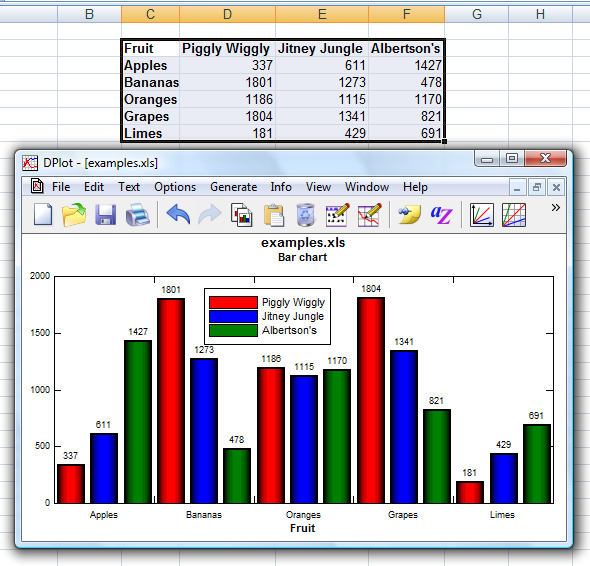
DPlot Windows software for Excel users to create presentation quality graphs

› documents › excelHow to rotate axis labels in chart in Excel? 3. Close the dialog, then you can see the axis labels are rotated. Rotate axis labels in chart of Excel 2013. If you are using Microsoft Excel 2013, you can rotate the axis labels with following steps: 1. Go to the chart and right click its axis labels you will rotate, and select the Format Axis from the context menu. 2.

data visualization - How do you put values over a simple bar chart in Excel? - Cross Validated

Edit titles or data labels in a chart - support.microsoft.com On a chart, click the label that you want to link to a corresponding worksheet cell. On the worksheet, click in the formula bar, and then type an equal sign (=). Select the worksheet cell that contains the data or text that you want to display in your chart. You can also type the reference to the worksheet cell in the formula bar.

How to edit the label of a chart in Excel? - Stack Overflow

Add or remove data labels in a chart - support.microsoft.com Click Label Options and under Label Contains, pick the options you want. Use cell values as data labels You can use cell values as data labels for your chart. Right-click the data series or data label to display more data for, and then click Format Data Labels. Click Label Options and under Label Contains, select the Values From Cells checkbox.

How to wrap X axis labels in a chart in Excel?

How to Add Labels to Scatterplot Points in Excel - Statology Next, click anywhere on the chart until a green plus (+) sign appears in the top right corner. Then click Data Labels, then click More Options… In the Format Data Labels window that appears on the right of the screen, uncheck the box next to Y Value and check the box next to Value From Cells.

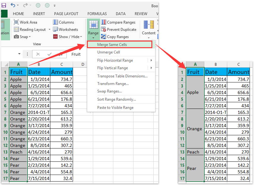
How to group (two-level) axis labels in a chart in Excel?

How to add or move data labels in Excel chart? In Excel 2013 or 2016. 1. Click the chart to show the Chart Elements button . 2. Then click the Chart Elements, and check Data Labels, then you can click the arrow to choose an option about the data labels in the sub menu. See screenshot: In Excel 2010 or 2007. 1. click on the chart to show the Layout tab in the Chart Tools group. See ...

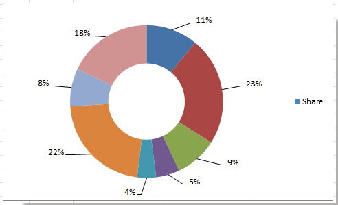
How to add leader lines to doughnut chart in Excel?

How to hide zero data labels in chart in Excel? - ExtendOffice Sometimes, you may add data labels in chart for making the data value more clearly and directly in Excel. But in some cases, there are zero data labels in the chart, and you may want to hide these zero data labels. Here I will tell you a quick way to hide the zero data labels in Excel at once. Hide zero data labels in chart

Excel Data Labels - Value from Cells

How to add data labels from different column in an Excel chart? This method will guide you to manually add a data label from a cell of different column at a time in an Excel chart. 1. Right click the data series in the chart, and select Add Data Labels > Add Data Labels from the context menu to add data labels. 2.

How to Handle Blank Cells in Excel | HowTech

chandoo.org › wp › change-data-labels-in-chartsHow to Change Excel Chart Data Labels to Custom Values? You can change data labels and point them to different cells using this little trick. First add data labels to the chart (Layout Ribbon > Data Labels) Define the new data label values in a bunch of cells, like this: Now, click on any data label. This will select "all" data labels. Now click once again.

How to Count Unique Values in Excel 2016? (with Pictures) - QueHow

› 509290 › how-to-use-cell-valuesHow to Use Cell Values for Excel Chart Labels Mar 12, 2020 · Select the chart, choose the “Chart Elements” option, click the “Data Labels” arrow, and then “More Options.” Uncheck the “Value” box and check the “Value From Cells” box. Select cells C2:C6 to use for the data label range and then click the “OK” button. The values from these cells are now used for the chart data labels.

Excel Variance Charts: Making Awesome Actual vs Target Or Budget Graphs - How To ...

Values From Cell: Missing Data Labels Option in Excel 2013? When a chart created in 2013 using the "Values from Cell" data label option is opened with any earlier version of Excel, the data labels will show as " [CELLRANGE]". In the formula bar enter a formula that points to the cell that holds the desired label. This process can be tedious for larger charts with many labels.

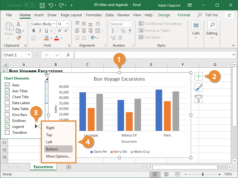
How to Edit a Legend in Excel | CustomGuide

How to link a cell to chart title/text box in Excel? 3. Go to the formula bar, and type the equal sign = into the formula bar, then select the cell you want to link to the chart title. See screenshot: 4. Press Enter key. Then you can see the selected cell is linked to chart title. Now when the cell A1 changes its contents, the chart title will automatically change.

How to Use Cell Values for Excel Chart Labels

Excel charts: add title, customize chart axis, legend and data labels ... Click the Chart Elements button, and select the Data Labels option. For example, this is how we can add labels to one of the data series in our Excel chart: For specific chart types, such as pie chart, you can also choose the labels location. For this, click the arrow next to Data Labels, and choose the option you want.

Ablebits.com Ultimate Suite for Excel - 60+ professional tools to get more power from your Excel

› charts › dynamic-chart-dataCreate Dynamic Chart Data Labels with Slicers - Excel Campus Feb 10, 2016 · Typically a chart will display data labels based on the underlying source data for the chart. In Excel 2013 a new feature called “Value from Cells” was introduced. This feature allows us to specify the a range that we want to use for the labels. Since our data labels will change between a currency ($) and percentage (%) formats, we need a ...

How to Delete blank cells in excel | Remove Blank rows & column