39 excel data labels from third column

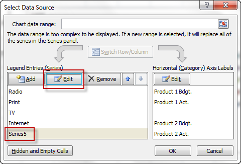
Change the format of data labels in a chart - support.microsoft.com Tip: To switch from custom text back to the pre-built data labels, click Reset Label Text under Label Options. To format data labels, select your chart, and then in the Chart Design tab, click Add Chart Element > Data Labels > More Data Label Options. Click Label Options and under Label Contains, pick the options you want. How to Change Excel Chart Data Labels to Custom Values? - Chandoo.org First add data labels to the chart (Layout Ribbon > Data Labels) Define the new data label values in a bunch of cells, like this: Now, click on any data label. This will select "all" data labels. Now click once again. At this point excel will select only one data label. Go to Formula bar, press = and point to the cell where the data label ...

How to create Custom Data Labels in Excel Charts - Efficiency 365 To customize it, click on the arrow next to Data Labels and choose More Options … Unselect the Value option and select the Value from Cells option. Choose the third column (without the heading) as the range. Now we have exactly what we want. Some labels may overlap the chart elements and they have a transparent background by default.

Excel data labels from third column

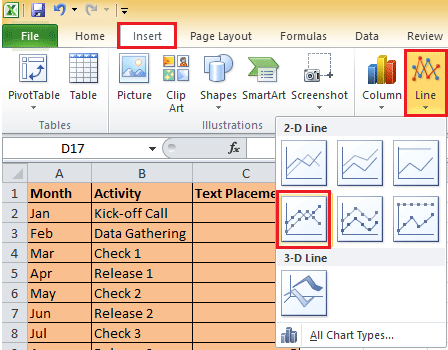
Custom data labels in a chart - Get Digital Help Press with right mouse button on on any data series displayed in the chart. Press with mouse on "Add Data Labels". Press with mouse on Add Data Labels". Double press with left mouse button on any data label to expand the "Format Data Series" pane. Enable checkbox "Value from cells". VLOOKUP Hack #4: Column Labels - Excel University This MATCH function would return 2 since the Amount label is in the 2nd table column. So, replacing the 2 in our original formula with the MATCH function would look like this: =VLOOKUP (B5, Table1, MATCH (C4,Table1 [#Headers],0), 0) This technique allows us to reference the column labels instead of the position number. But, Jeff, hang on. How to add data labels to a Column (Vertical Bar) Graph in ... - YouTube Get to know about easy steps to add data labels to a Column (Vertical Bar) Graph in Microsoft® Excel 2010 by watching this video.Content in this video is pro...

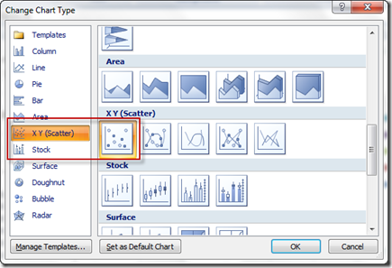
Excel data labels from third column. Adding rich data labels to charts in Excel 2013 - microsoft.com Putting a data label into a shape can add another type of visual emphasis. To add a data label in a shape, select the data point of interest, then right-click it to pull up the context menu. Click Add Data Label, then click Add Data Callout . The result is that your data label will appear in a graphical callout. How can I add data labels from a third column to a scatterplot? Do you want to add data labels to the 3rd column values in the chart? Highlight the 3rd column range in the chart. Click the chart, and then click the Chart Layout tab. Under Labels, click Data Labels, and then in the upper part of the list, click the data label type that you want. Steps to Print Labels from Excel - EDUCBA Navigate towards the folder where the excel file is stored in the Select Data Source pop-up window. Select the file in which the labels are stored and click Open. A new pop up box named Confirm Data Source will appear. Click on OK to let the system know that you want to use the data source. Again a pop-up window named Select Table will appear. Add or remove data labels in a chart - support.microsoft.com Right-click the data series or data label to display more data for, and then click Format Data Labels. Click Label Options and under Label Contains, select the Values From Cells checkbox. When the Data Label Range dialog box appears, go back to the spreadsheet and select the range for which you want the cell values to display as data labels.

How to add data labels from different column in an Excel chart? This method will guide you to manually add a data label from a cell of different column at a time in an Excel chart. 1. Right click the data series in the chart, and select Add Data Labels > Add Data Labels from the context menu to add data labels. 2. How to Add Labels to Scatterplot Points in Excel - Statology Next, click anywhere on the chart until a green plus (+) sign appears in the top right corner. Then click Data Labels, then click More Options… In the Format Data Labels window that appears on the right of the screen, uncheck the box next to Y Value and check the box next to Value From Cells. Apply Custom Data Labels to Charted Points - Peltier Tech Click once on a label to select the series of labels. Click again on a label to select just that specific label. Double click on the label to highlight the text of the label, or just click once to insert the cursor into the existing text. Type the text you want to display in the label, and press the Enter key. Mac Excel 2008 - How to add Data Labels for Scatter Plot coming from ... In Excel 2008, to select X axis for the labels: go to 'Formatting palette' navigate to 'Chart Option' Under 'Other options' select "category name' in Labels. A AsherS New Member Joined Feb 9, 2012 Messages 9 Jul 30, 2014 #3 Cyrilbrd, this does not add a label from another column. This only displays the X-value and does not solve the issue. cyrilbrd

How to Print Labels from Excel Using Database Connections - TEKLYNX Open label design software. Click on Data Sources, and then click Create/Edit Query. Select Excel and name your database. Browse and attach your database file. Save your query so it can be used again in the future. Select the necessary fields (columns) that you would like to use on your label template. 😊. How to compare two columns and return values from the third column in ... The entire Column C items in Sheet 2 to be compared with first row item in Column A and if any corresponding values/data are there in Column A, then Column B to be populated with data corresponding to the row item in Column D. Column C will have a single word. Column D may or may not have data in it. Column A will have more text. Excel, giving data labels to only the top/bottom X% values 1) Create a data set next to your original series column with only the values you want labels for (again, this can be formula driven to only select the top / bottom n values). See column D below. 2) Add this data series to the chart and show the data labels. 3) Set the line color to No Line, so that it does not appear! 4) Volia! See Below! Share Using a cell contents of a third column of data as data label for each ... Column 1 is a numeric value for an ion and is on the X-axis, column 2 is a numerical value for intensity at the value of column 1. Column 3 is a text descriptor of what type of ion gives that column 1 reading value and its column 2 intensity value. I would like to use the column 3 data to label each column on the chart above the column.

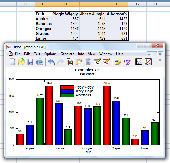
DPlot Windows software for Excel users to create presentation quality graphs

Excel VBA - Add Data Labels from Table body range Sub InsertLabelnameBubble () ActiveChart.FullSeriesCollection (1).DataLabels.Select For i = 1 To Range ("Table").Rows.Count ActiveChart.FullSeriesCollection (1).Points (i).DataLabel.Select Selection.Formula = Range ("Table").Cells (i, 1) Next i End Sub Here's a screenshot of my project.

How-to Add Centered Labels Above an Excel Clustered Stacked Column Chart - Excel Dashboard Templates

Create a multi-level category chart in Excel - ExtendOffice 1.3) In the third column, type in each data for the subcategories. 2. Select the data range, click Insert > Insert Column or Bar Chart > Clustered Bar. 3. Drag the chart border to enlarge the chart area. See the below demo. 4. Right click the bar and select Format Data Series from the right-clicking menu to open the Format Data Series pane.

How to create a timeline milestone chart in Excel?

Using Data Labels from a Third Data Column in an Chart - Chandoo.org Excel 2013, allows you to select Data Labels locations from a Dialog box Prior to that it had to be done either manually or via a Macro To do it manually Select a Series Add a Data Label Select the Data Labels Then select an Individual Data Label In the formula bar =$D$2 (Cell reference to your new labels) Repeat for all Labels G guna_sekar87

How-to Add Centered Labels Above an Excel Clustered Stacked Column Chart - Excel Dashboard Templates

Custom Data Labels with Colors and Symbols in Excel Charts - [How To] Step 4: Select the data in column C and hit Ctrl+1 to invoke format cell dialogue box. From left click custom and have your cursor in the type field and follow these steps: Press and Hold ALT key on the keyboard and on the Numpad hit 3 and 0 keys. Let go the ALT key and you will see that upward arrow is inserted.

SQL Workbench/J User's Manual SQLWorkbench

How to Use Cell Values for Excel Chart Labels - How-To Geek Make your chart labels in Microsoft Excel dynamic by linking them to cell values. When the data changes, the chart labels automatically update. In this article, we explore how to make both your chart title and the chart data labels dynamic. We have the sample data below with product sales and the difference in last month's sales.

Share :