44 excel pivot table 2 row labels

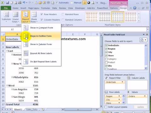
Pivot table row labels in separate columns • AuditExcel.co.za Our preference is rather that the pivot tables are shown in tabular form (all columns separated and next to each other). You can do this by changing the report format. So when you click in the Pivot Table and click on the DESIGN tab one of the options is the Report Layout. Click on this and change it to Tabular form. Combining two+ Columns to form one Row label column in Pivot Table Re: Combining two+ Columns to form one Row label column in Pivot Table Select a cell in your pivot table. Press Alt, then D, then P (i.e. in succession; not all at the same time), to call up the Pivot Table Wizard. Click "" button twice.

How To Repeat Row Labels In Pivot Table Free Excel Tutorial If you want to Save How To Repeat Row Labels In Pivot Table Free Excel Tutorial with original size you can click the Download link. One Piece Tempo X2 Tier List Maker, Gpo Value Tier List Tier List Maker, Printable Sudoku Sudoku Printable Free Printable Sudoku, How To Repeat Row Labels In Pivot Table Free Excel Tutorial, ...

Excel pivot table 2 row labels

Design the layout and format of a PivotTable Change a PivotTable to compact, outline, or tabular form Change the way item labels are displayed in a layout form Change the field arrangement in a PivotTable Add fields to a PivotTable Copy fields in a PivotTable Rearrange fields in a PivotTable Remove fields from a PivotTable Change the layout of columns, rows, and subtotals Use column labels from an Excel table as the rows in a Pivot Table ... Highlight your current table, including the headers Then from the Data section of the ribbon, select From Table Highlight all the columns containing data, but not the Year column, and then select Unpivot Columns Close the dialog and keep the changes. Excel should place the unpivoted data into a new worksheet, looking something like this: Automatic Row And Column Pivot Table Labels - How To Excel At Excel Select the data set you want to use for your table The first thing to do is put your cursor somewhere in your data list Select the Insert Tab Hit Pivot Table icon Next select Pivot Table option Select a table or range option Select to put your Table on a New Worksheet or on the current one, for this tutorial select the first option Click Ok

Excel pivot table 2 row labels. Data Labels in Excel Pivot Chart (Detailed Analysis) 7 Suitable Examples with Data Labels in Excel Pivot Chart Considering All Factors 1. Adding Data Labels in Pivot Chart 2. Set Cell Values as Data Labels 3. Showing Percentages as Data Labels 4. Changing Appearance of Pivot Chart Labels 5. Changing Background of Data Labels 6. Dynamic Pivot Chart Data Labels with Slicers 7. Repeat item labels in a PivotTable - support.microsoft.com Right-click the row or column label you want to repeat, and click Field Settings. Click the Layout & Print tab, and check the Repeat item labels box. Make sure Show item labels in tabular form is selected. Notes: When you edit any of the repeated labels, the changes you make are applied to all other cells with the same label. Pivot Table adding "2" to value in answer set 1) Right click your pivot table -> Pivot table options -> Data -> Change "Number of items to retain per field" to NONE 2) Wipe all rows in your data source except for the headers 3) Refresh the pivot table 4) Save, and close all instances of Excel 5) Reopen the file, and paste your data 6) Refresh the pivot table How to Add Rows to a Pivot Table: 9 Steps (with Pictures) - wikiHow Click anywhere in your pivot table. This opens the pivot table editor on the right side of Google Sheets. 3. Click Add under "Rows." It's in the left side of the pivot table editor. A list of fields will expand on the menu. 4. Click the name of the field you want to add as a row.

Excel, Pivot and multiple row labels - Super User where "Server" and "Version" are always the same in a row. I would like a pivot table with | Server | Version | DBs | | a | v1 | 3 | | b | v2 | 2 | with DBs as the number of DBs on the given server. Now I only manage to have one column "Server" as Row label. If I add the "Version" column to the list of columns I get something like How to rename group or row labels in Excel PivotTable? - ExtendOffice You can rename a group name in PivotTable as to retype a cell content in Excel. Click at the Group name, then go to the formula bar, type the new name for the group. Rename Row Labels name To rename Row Labels, you need to go to the Active Field textbox. 1. Click at the PivotTable, then click Analyze tab and go to the Active Field textbox. 2. While in the visual basic editor, go the Tools menu and select ... To format data labels in Excel, choose the. To create an Excel pivot table, Open your original spreadsheet and remove any blank rows or columns. You may also use the Excel sample data at the bottom of this tutorial. Make sure each column has a meaningful label. The column labels will be carried over to the Field List. Right-click the table and How to Group Rows in Excel Pivot Table (3 Ways) - ExcelDemy Now select any number in the Row Labels of the table. Then right-click and select Group as shown below. Then, enter the Starting ( 60) and Ending ( 100) numbers and the difference ( 10) by which you want to group them. Next, hit OK. Finally, you will see the numbers grouped together as shown in the picture below.👇.

Excel Pivot Table Row labels - Stack Overflow 1 Answer. Right click on the pivot, go to PivotTable Options, Display Tab. Click on "Classic Pivot Table Layout". Go to each field (column), right click, field settings, layout & print tab. Click on "Repeat Item Labels". That should give you the table you're looking for. Sep 11, 2014 - mcsznj.implanty-michno.pl Step 2: Create the Pivot Table. Next, create a pivot table, with the field you want to group on as a row label. In our example, we are going to use the price as the row label, and the number (count) of transactions in the value area. As you can see from the picture below, our resulting pivot table has individual prices. Description Consists of - gct.gimnazjummrocza.pl Step 2: Create the Pivot Table. Next, create a pivot table, with the field you want to group on as a row label. In our example, we are going to use the price as the row label, and the number (count) of transactions in the value area. As you can see from the picture below, our resulting pivot table has individual prices. This pivot table shows a ... Multiple row labels on one row in Pivot table - MrExcel Message Board I figured it out - Right click on your pivot table and choose pivot table options/display. Click on "Classic PivotTable layout" Then click on where it is subtotaling your row label and uncheck the subtotal option. D dudeshane0 New Member Joined Oct 23, 2014 Messages 1 Jan 19, 2015 #6 Gerald Higgins said:

How to Sort Data in a Pivot Table | Excelchat

Pivot Table "Row Labels" Header Frustration Pivot Table "Row Labels" Header Frustration. Hi Everyone please help I can't change my headers from Row Labels in a Pivot Table. Using Excel 365. Labels:

Repeat Headings in Excel 2010 Pivot Table - YouTube

How to make row labels on same line in pivot table? - ExtendOffice Make row labels on same line with setting the layout form in pivot table As we all know, the pivot table has several layout form, the tabular form may help us to put the row labels next to each other. Please do as follows: 1. Click any cell in your pivot table, and the PivotTable Tools tab will be displayed. 2.

Excel Help: Simple method to make Pivot table

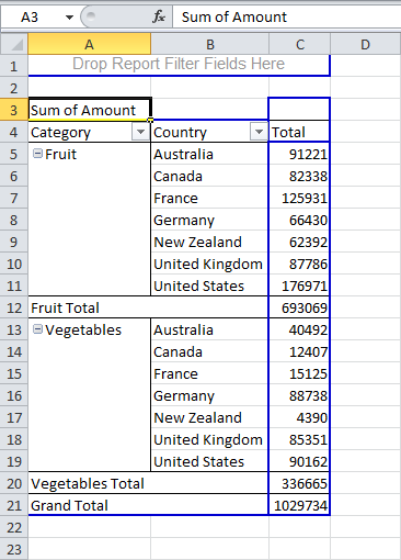
Pivot table row labels side by side - Excel Tutorials - OfficeTuts Excel You can copy the following table and paste it into your worksheet as Match Destination Formatting. Now, let's create a pivot table ( Insert >> Tables >> Pivot Table) and check all the values in Pivot Table Fields. Fields should look like this. Right-click inside a pivot table and choose PivotTable Options…. Check data as shown on the image below.

How to Know the Pivot Field Orientation in Excel Pivot Table with VBA | Microsoft Power BI Kingdom

Excel Pivot Table with nested rows | Basic Excel Tutorial Insert your pivot table. Click Insert Menu, under Tables group choose PivotTable. 2. Once you create your pivot table, add all the fields you need to analyze data. How to add the fields. Select the checkbox on each field name you desire in the field section. The selected fields are added to the Row Labels area in the layout section.

Can I use the union of two columns values in Excel as row labels in a Pivot Table? - Super User

get a row label from pivot table - Microsoft Tech Community Create PivotTable and after that convert it to cube formulas. Now you may take these formulas and convert it to form you need, for example. in H3 it could be. =CUBEVALUE( "ThisWorkbookDataModel", CUBEMEMBER("ThisWorkbookDataModel", " [Measures].

How to make row labels on same line in pivot table?

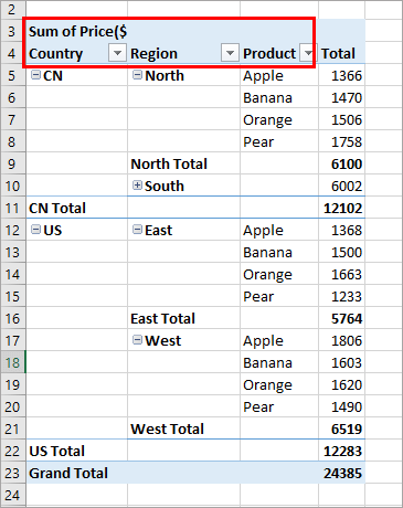
Pivot Table Row Labels In the Same Line - Beat Excel! First make a pivot table with required fields. Arrange the fields as shown in left picture. Your initial table will look like right picture. Now click on "Error Code" and access field settings. First check "None" option in "Subtotals & Filters" tab to disable totals after every row.

Design your Pivot Table in Excel | Excel in Excel

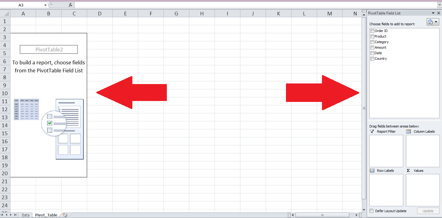
Multi-level Pivot Table in Excel - Excel Easy First, insert a pivot table. Next, drag the following fields to the different areas. 1. Order ID to the Rows area. 2. Amount field to the Values area. 3. Country field and Product field to the Filters area. 4. Next, select United Kingdom from the first filter drop-down and Broccoli from the second filter drop-down.

How to Use Excel in 2017: 14 Simple Excel Shortcuts, Tips & Tricks

Pivot Table Sort by second row label - Microsoft Community Ramz Aftab Replied on May 17, 2014 Here is how you can get the results: Place your cursor on Col. B data wherever Names are. Goto Home ribbon>Editing>Sort it in either way. Alternatively, you can Sort from Pivots settings. Ramz Aftab [ MOS 77-888/82 Excel Expert ] ramzaftab [at]gmail [.]com Report abuse Was this reply helpful? Yes No

How to use a pivot table in Excel 2013 - Quora

Tableau is one of the leading business intelligence tools used ... Here are the steps for creating a pivot table: Select the data on the spreadsheet you want to include in the table. On the Excel ribbon go to Insert > Tables > Pivot table. A Create PivotTable dialog box will appear, with the data range you selected. You can manually edit the data range as you see fit. Figure 6 - How to sort pivot table date ...

Multiple Row Fields

How to Use Excel Pivot Table Label Filters - Contextures Excel Tips Right-click a cell in the pivot table, and click PivotTable Options. In the PivotTable Options dialog box, click the Totals & Filters tab. In the Filters section, add a check mark to 'Allow multiple filters per field.'. Click the OK button, to apply the setting and close the dialog box.

23 things you should know about Excel pivot tables | Exceljet

Remove PivotTable Duplicate Row Labels [SOLVED] Re: Remove PivotTable Duplicate Row Labels Sometimes when the cells are stored in different formats within the same column in the raw data, they get duplicated. Also, if there is space/s at the beginning or at the end of these fields, when you filter them out they look the same, however, when you plot a Pivot Table, they appear as separate headers.

Create a Pivot Table in Excel - The Complete Beginners Guide - QuickExcel

How to Customize Your Excel Pivot Chart Data Labels The Data Labels command on the Design tab's Add Chart Element menu in Excel allows you to label data markers with values from your pivot table. When you click the command button, Excel displays a menu with commands corresponding to locations for the data labels: None, Center, Left, Right, Above, and Below.

Pivot Table Row Labels Side By Side | Decorations I Can Make

Automatic Row And Column Pivot Table Labels - How To Excel At Excel Select the data set you want to use for your table The first thing to do is put your cursor somewhere in your data list Select the Insert Tab Hit Pivot Table icon Next select Pivot Table option Select a table or range option Select to put your Table on a New Worksheet or on the current one, for this tutorial select the first option Click Ok

Excel pivot table hides complete row when blank values or labels are filtered - Super User

Use column labels from an Excel table as the rows in a Pivot Table ... Highlight your current table, including the headers Then from the Data section of the ribbon, select From Table Highlight all the columns containing data, but not the Year column, and then select Unpivot Columns Close the dialog and keep the changes. Excel should place the unpivoted data into a new worksheet, looking something like this: