43 data labels excel pie chart
How to Create and Format a Pie Chart in Excel - Lifewire Select the plot area of the pie chart. Select a slice of the pie chart to surround the slice with small blue highlight dots. Drag the slice away from the pie chart to explode it. To reposition a data label, select the data label to select all data labels. Select the data label you want to move and drag it to the desired location. 45 Free Pie Chart Templates (Word, Excel & PDF) ᐅ TemplateLab 45 Free Pie Chart Templates (Word, Excel & PDF) ... Edit each of the labels by typing the categories of your data. Edit the chart’s title by clicking on it and inputting the title. Replace each of the values next to each of the labels according to your data. Drawing your pie chart template
Add or remove data labels in a chart - support.microsoft.com Data labels make a chart easier to understand because they show details about a data series or its individual data points. For example, in the pie chart below, without the data labels it would be difficult to tell that coffee was 38% of total sales. Depending on what you want to highlight on a chart, you can add labels to one series, all the ...
Data labels excel pie chart
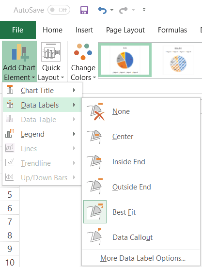
Excel Pie Chart - How to Create & Customize? (Top 5 Types) The steps to add percentages to the Pie Chart are: Step 1: Click on the Pie Chart > click the ' + ' icon > check/tick the " Data Labels " checkbox in the " Chart Element " box > select the " Data Labels " right arrow > select the " More Options… ", as shown below. Step 2: The Format Data Labels pane opens. Move data labels - support.microsoft.com Right-click the selection > Chart Elements > Data Labels arrow, and select the placement option you want. Different options are available for different chart types. For example, you can place data labels outside of the data points in a pie chart but not in a column chart. Edit titles or data labels in a chart - support.microsoft.com On a chart, click one time or two times on the data label that you want to link to a corresponding worksheet cell. The first click selects the data labels for the whole data series, and the second click selects the individual data label. Right-click the data label, and then click Format Data Label or Format Data Labels.
Data labels excel pie chart. How To Make A Pie Chart In Excel: In Just 2 Minutes [2022] When you first create a pie chart, Excel will use the default colors and design.. But if you want to customize your chart to your own liking, you have plenty of options. The easiest way to get an entirely new look is with chart styles.. In the Design portion of the Ribbon, you’ll see a number of different styles displayed in a row. Mouse over them to see a preview: › examples › pie-chartCreate a Pie Chart in Excel (In Easy Steps) - Excel Easy 6. Create the pie chart (repeat steps 2-3). 7. Click the legend at the bottom and press Delete. 8. Select the pie chart. 9. Click the + button on the right side of the chart and click the check box next to Data Labels. 10. Click the paintbrush icon on the right side of the chart and change the color scheme of the pie chart. Result: 11. Excel pie chart from list of names - KarissAiyla Create Multiple Pie Charts In Excel Using Worksheet Data And Vba Pie Charts Pie Chart Pie Chart Template ... Right-click the pie chart and expand the add data labels option. Sub SlicesColors Dim chtO As ChartObject Dim ser As Series Dim clf As ColorFormat Dim j. A pie chart comprises of slices each of which represents a given value in the form ... Pie Chart in Excel - Inserting, Formatting, Filters, Data Labels Adding Data Labels. The default pie chart inserted in the above section is:-. From this chart, we can come up to applications usage order, but can't read the exact contributions. To add Data Labels, Click on the + icon on the top right corner of the chart and mark the data label checkbox.
Display data point labels outside a pie chart in a paginated report ... Create a pie chart and display the data labels. Open the Properties pane. On the design surface, click on the pie itself to display the Category properties in the Properties pane. Expand the CustomAttributes node. A list of attributes for the pie chart is displayed. Set the PieLabelStyle property to Outside. Set the PieLineColor property to Black. The PieLineColor property defines callout lines for each data point label. To prevent overlapping labels displayed outside a pie chart. Create a ... How to Show Percentage in Pie Chart in Excel? - GeeksforGeeks 29/06/2021 · Select a 2-D pie chart from the drop-down. A pie chart will be built. Select -> Insert -> Doughnut or Pie Chart -> 2-D Pie. Initially, the pie chart will not have any data labels in it. To add data labels, select the chart and then click on the “+” button in the top right corner of the pie chart and check the Data Labels button. How to Make a Pie Chart with Multiple Data in Excel (2 Ways) - ExcelDemy First, select the entire data set and go to the Insert tab from the ribbon. After that, choose Insert Pie and Doughnut Chart from the Charts group. Afterward, click on the 2nd Pie Chart among the 2-D Pie as marked on the following picture. Now, Excel will instantly create a Pie of Pie Chart in your worksheet. why are some data labels not showing in pie chart ... - Power BI Hi @Anonymous. Enlarge the chart, change the format setting as below. Details label->Label position: perfer outside, turn on "overflow text". For donut charts, you could refer to the following thread: How to show all detailed data labels of donut chart. Best Regards.
How to hide zero data labels in chart in Excel? - ExtendOffice 1. Right click at one of the data labels, and select Format Data Labels from the context menu. See screenshot: 2. In the Format Data Labels dialog, Click Number in left pane, then select Custom from the Category list box, and type #"" into the Format Code text box, and click Add button to add it to Type list box. See screenshot: 3. How to display leader lines in pie chart in Excel? - ExtendOffice To display leader lines in pie chart, you just need to check an option then drag the labels out. 1. Click at the chart, and right click to select Format Data Labels from context menu. 2. In the popping Format Data Labels dialog/pane, check Show Leader Lines in the Label Options section. See screenshot: 3. Close the dialog, now you can see some ... pie chart - Hide a range of data labels in 'pie of pie' in Excel ... First format the second pie so that each slice has no fill (becomes invisible), to speed this up just set the first slice to no fill and then highlight each slice and select F4 to repeat last action. Next select any slice from the main chart and hit CTRL+1 to bring up the Series Option window, here set the gap width to 0% (this will centre the ... › pie-chart-examplesPie Chart Examples | Types of Pie Charts in Excel with Examples It is similar to Pie of the pie chart, but the only difference is that instead of a sub pie chart, a sub bar chart will be created. With this, we have completed all the 2D charts, and now we will create a 3D Pie chart. 4. 3D PIE Chart. A 3D pie chart is similar to PIE, but it has depth in addition to length and breadth.
How to Create Excel Pie Charts & Add Rich Data Labels to The Chart!
› ms-excel-pie-chartHow to Make a Pie Chart in Excel (Only Guide You Need) Jul 13, 2022 · Read More: How to Make Pie Chart in Excel with Subcategories (2 Quick Methods) Conclusion. Hope after reading this article you will not face any difficulties with the pie chart. This article covers all the necessary things regarding Excel Pie Chart. Stay tuned for more useful articles. Let us know what problems do you face with Excel Pie Chart.
How to Make a Pie Chart in Excel & Add Rich Data Labels to The Chart!
How to Edit Pie Chart in Excel (All Possible Modifications) How to Edit Pie Chart in Excel 1. Change Chart Color 2. Change Background Color 3. Change Font of Pie Chart 4. Change Chart Border 5. Resize Pie Chart 6. Change Chart Title Position 7. Change Data Labels Position 8. Show Percentage on Data Labels 9. Change Pie Chart's Legend Position 10. Edit Pie Chart Using Switch Row/Column Button 11.

33 How To Label Pie Chart In Excel - Labels Design Ideas 2020
spreadsheeto.com › pie-chartHow To Make A Pie Chart In Excel. - Spreadsheeto How To Make A Pie Chart In Excel. In Just 2 Minutes! Written by co-founder Kasper Langmann, Microsoft Office Specialist. The pie chart is one of the most commonly used charts in Excel. Why? Because it’s so useful 🙂. Pie charts can show a lot of information in a small amount of space. They primarily show how different values add up to a whole.

410 How to display percentage labels in pie chart in Excel 2016 - YouTube
Add data labels and callouts to charts in Excel 365 - EasyTweaks.com Step #2: When you select the "Add Labels" option, all the different portions of the chart will automatically take on the corresponding values in the table that you used to generate the chart. The values in your chat labels are dynamic and will automatically change when the source value in the table changes. Step #3: Format the data labels.

SQL & BI Learning: Pie Chart with data labels outside in ssrs
support.microsoft.com › en-us › officeAdd or remove data labels in a chart - support.microsoft.com Data labels make a chart easier to understand because they show details about a data series or its individual data points. For example, in the pie chart below, without the data labels it would be difficult to tell that coffee was 38% of total sales. Depending on what you want to highlight on a chart, you can add labels to one series, all the ...

Lesson 38 - How to add DATA LABELS to charts in Excel | Change colour of pie-chart segments in ...
Pie Chart Examples | Types of Pie Charts in Excel with Examples Now our task is to add the Data series to the PIE chart divisions. Popular Course in this category. Excel Training (21 Courses, ... Right-click and choose the “Add Data Labels “option for additional drop-down options. From that drop-down, select the option “Add Data Callouts”. ... Here we discuss Types of Pie Chart in Excel along with ...

Python matplotlib Pie Chart
How to create a pie chart in Microsoft Excel Remember that when a user changes the pie chart data, it will automatically update. Create basic pie chart. You can create pie charts in two different ways and both start by selecting cells. Be sure to select only the cells you want to convert into a chart. Method 1. Select the cells, right-click the selected group and select Quick Analysis ...
How to Make a Pie Chart in Excel & Add Rich Data Labels to The Chart!
Pie Chart in Excel | How to Create Pie Chart - EDUCBA Step 1: Do not select the data; rather, place a cursor outside the data and insert one PIE CHART. Go to the Insert tab and click on a PIE. Step 2: once you click on a 2-D Pie chart, it will insert the blank chart as shown in the below image. Step 3: Right-click on the chart and choose Select Data.
How to Show Percentages in Stacked Bar and Column Charts in Excel
How to Make a Pie Chart in Excel (Only Guide You Need) 13/07/2022 · Read More: How to Make Pie Chart in Excel with Subcategories (2 Quick Methods) Conclusion. Hope after reading this article you will not face any difficulties with the pie chart. This article covers all the necessary things regarding Excel Pie Chart. Stay tuned for more useful articles. Let us know what problems do you face with Excel Pie Chart.
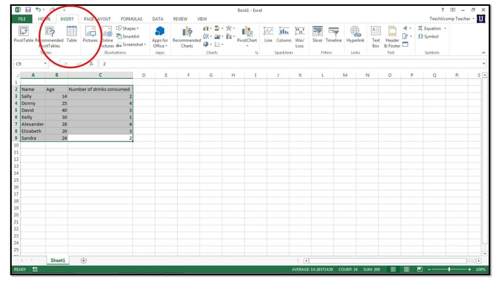
How to Insert Charts into an Excel Spreadsheet in Excel 2013
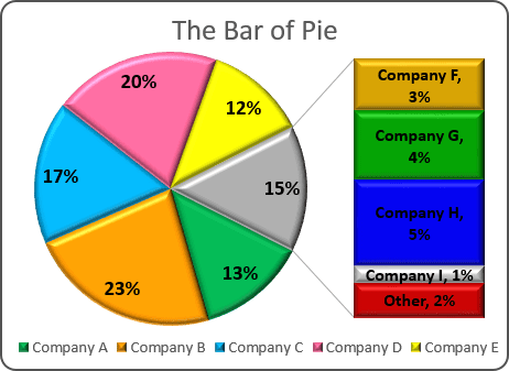
How to Create Bar of Pie Chart in Excel? Step-by-Step The Bar of Pie chart is quite flexible, in that you can adjust the number of slices that you want to move from the main pie to the bar. Besides this, the Bar of pie chart in Excel calculates and displays percentages of each category automatically as data labels, so you don’t need to worry about calculating the portion sizes yourself.
33 How To Label Pie Chart In Excel - Labels Design Ideas 2020
How to display leader lines in pie chart in Excel? - ExtendOffice To display leader lines in pie chart, you just need to check an option then drag the labels out. 1. Click at the chart, and right click to select Format Data Labels from context menu. 2. In the popping Format Data Labels dialog/pane, check Show Leader Lines in the Label Options section. See screenshot: 3.
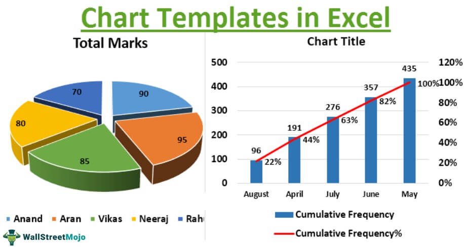
Chart Templates in Excel | 10 Steps to Create Excel Chart Template
spreadsheetplanet.com › bar-of-pie-chart-excelHow to Create Bar of Pie Chart in Excel? Step-by-Step The Bar of Pie chart is quite flexible, in that you can adjust the number of slices that you want to move from the main pie to the bar. Besides this, the Bar of pie chart in Excel calculates and displays percentages of each category automatically as data labels, so you don’t need to worry about calculating the portion sizes yourself.
Creating Pie of Pie and Bar of Pie charts - Microsoft Excel 2016
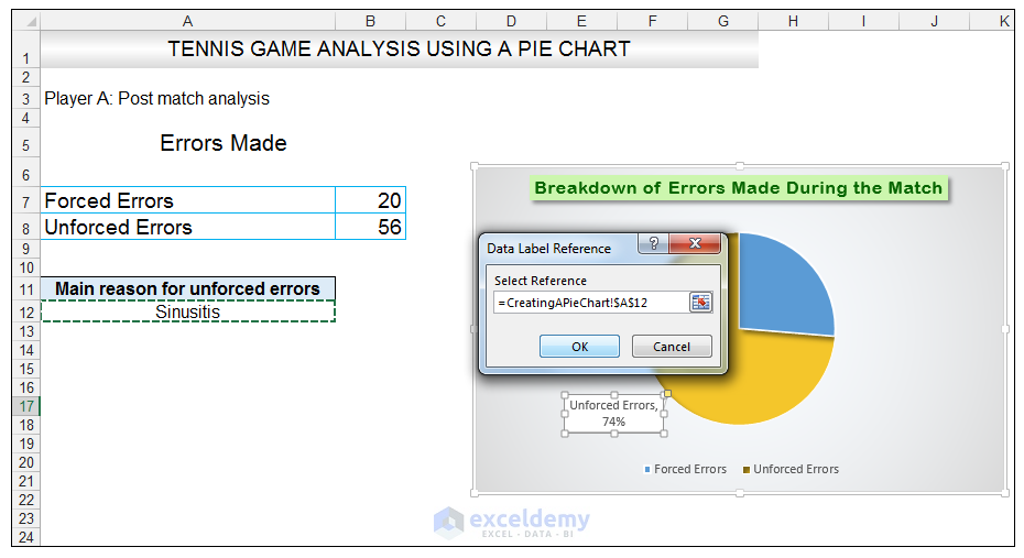
support.microsoft.com › en-us › officeChange the format of data labels in a chart You can add a built-in chart field, such as the series or category name, to the data label. But much more powerful is adding a cell reference with explanatory text or a calculated value. Click the data label, right click it, and then click Insert Data Label Field. If you have selected the entire data series, you won't see this command.

Formatting data labels and printing pie charts on Excel for Mac 2019 - - Microsoft Community
Change the format of data labels in a chart Excel for Microsoft 365 Word for Microsoft 365 Outlook for Microsoft 365 PowerPoint for Microsoft 365 Excel ... Data labels make a chart easier to understand because they show details about a data series or its individual data points. For example, in the pie chart below, without the data labels it would be difficult to tell that coffee was 38% ...
How to Make a Pie Chart in Excel & Add Rich Data Labels to The Chart!
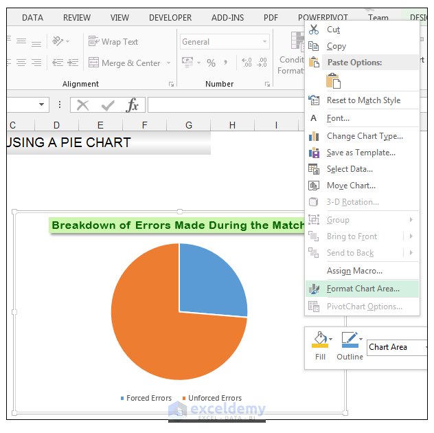
How to Make a Pie Chart in Excel & Add Rich Data Labels to The Chart! Creating and formatting the Pie Chart 1) Select the data. 2) Go to Insert> Charts> click on the drop-down arrow next to Pie Chart and under 2-D Pie, select the Pie Chart, shown below. 3) Chang the chart title to Breakdown of Errors Made During the Match, by clicking on it and typing the new title.

r - labels on the pie chart for small pieces (ggplot) - Stack Overflow
Multiple pie charts in one graph excel - SiamaEiliyah Right-click the pie chart and expand the add data labels option. In this video you will learn how to make multiple pie chart using two sets of data using Microsoft excel. ... You can easily generate a pie chart using two data. Multiple Pie Chart In Excel You may create a multiplication graph or chart in Stand out through a template. Every time ...
Excel 3-D Pie charts - Microsoft Excel 2013
Create a Pie Chart in Excel (In Easy Steps) - Excel Easy 6. Create the pie chart (repeat steps 2-3). 7. Click the legend at the bottom and press Delete. 8. Select the pie chart. 9. Click the + button on the right side of the chart and click the check box next to Data Labels. 10. Click the paintbrush icon on the right side of the chart and change the color scheme of the pie chart. Result: 11.
Post a Comment for "43 data labels excel pie chart"